Static Program Analysis

Book: https://users-cs.au.dk/amoeller/spa/

Applications

• Optimization
• Correctness
• Development

The input/behavior of nontrivial programs are undecidable.

The Tiny Imperative Language

• Syntax
• Normalization
• AST
• CFG

Type Analysis

Type -> int
      | ↑Type
      | (Type, ..., Type) -> Type

      // Infinite types (caused by recursion)
      | μ TypeVar. Type
      | TypeVar

      // Record
      | { Id: Type, ..., Id: Type }
      | ◊  // Absent field

TypeVar -> t | u | ...

Polymorphic + recursive = undecidable type analysis.

Limits:

• flow-sensitive
• polymorphic
• ignores other kinds of runtime errors

Lattice Theory

Partially ordered set

• Reflexive
• Transitive
• Antisymmetric

Lattice

• Least upper bound (join)
• Greatest lower bound (meet)

Complete lattice: every subset has a join and a meet.

• Top $\mathrm{\top }$
• Bottom $\mathrm{\perp }$

Examples:

• Powerset lattice $(\mathcal{P}(S),\subseteq )$
• Flat lattice $\text{flat}(A)$
• Product lattice $L_1\times L_2$
• Function lattice $L_1\to L_2$

Homomorphism:

• Homomorphism: $f:L_1\to L_2$ such that $f(x\bigsqcup y)=f(x)\bigsqcup f(y)\wedge f(x\sqcap y)=f(x)\sqcap f(y)$
• Isomorphism = bijective homomorphism

$\text{lift}(L)$: $L$ with a new bottom element

Equation System:

fixed point, least fixed point (LFP)

For monotonic function $f:L\to L$, $\text{LFP}(f)={\bigsqcup }_{i=0}^{\mathrm{\infty }}{f}^i(\mathrm{\perp })$

Dataflow Analysis with Monotone Frameworks

Sign analysis, Constant propagation analysis:

• $\text{JOIN}(v)={\bigsqcup }_{w\in \text{pred}(v)}[[w]]$
• X=E: $[[v]]=\text{JOIN}(v)[X\mapsto \text{eval}(\text{JOIN}(v),E)]$
• var X: $[[v]]=\text{JOIN}(v)[X\mapsto \mathrm{\top }]$

Live variable analysis:

• $\text{JOIN}(v)={\cup }_{w\in \text{succ}(v)}[[w]]$
• X=E: $[[v]]=\text{JOIN}(v)\setminus \{X\}\cup \text{vars}(E)$
• if (E), output E: $[[v]]=\text{JOIN}(v)\cup \text{vars}(E)$
• var X: $[[v]]=\text{JOIN}(v)\setminus \{X\}$
• exit: $[[v]]=\mathrm{\varnothing }$

Available expressions analysis:

• State = (P({exprs}), $\subseteq$)
• $\text{JOIN}(v)={\cap }_{w\in \text{pred}(v)}[[w]]$
• X=E: $[[v]]=\text{JOIN}(v)\cup \{E\}$ removed all expressions that contain $X$
• if (E), output E: $[[v]]=\text{JOIN}(v)\cup \{E\}$

Very busy expressions analysis:

• $\text{JOIN}(v)={\cap }_{w\in \text{succ}(v)}[[w]]$
• X=E: $[[v]]=\text{JOIN}(v)$ removed all expressions that contain $X\cup \{E\}$
• Usage: "Code hoisting"

Reaching definitions analysis:

• State = (P({definitions}), $\subseteq$)
• $\text{JOIN}(v)={\cup }_{w\in \text{pred}(v)}[[w]]$
• X=E: $[[v]]=\text{JOIN}(v)\downarrow \{X\}\cup \{v\}$
• Usage: "DCE", "Code motion"

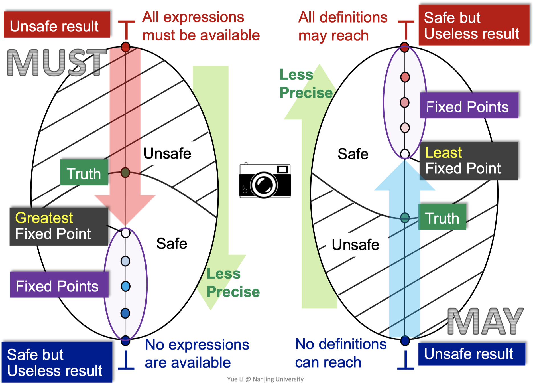
Summary

	Forward	Backward
May	Reaching definitions	Live variables
Must	Available expressions	Very busy expressions

Transfer function: $[[v]]=t_v(\text{JOIN}(v))$

Widening and Narrowing

• Allowing lattices with infinite height to converge.
• Accelerate finite height lattices.

1. Widening: $B$
2. Narrowing: Not guaranteed to converge. Heuristics must determine how many iterations to apply.

Widening operator: $\mathrm{\nabla }:L\times L\to L$:

• Only apply widening at recursive dataflow constraints.

Path Sensitivity

Assertions: $\mathtt{\text{assert}}(E)$

• Trivial: $[[\mathtt{\text{assert}}(E)]]=\text{JOIN}(v)$
• Predicates: $[[\mathtt{\text{assert}}(E>0)]]=\text{JOIN}(v)[X\mapsto \text{gt}(\text{JOIN}(v)(X),\text{eval}(\text{JOIN}(v),E))]$
• Sound & Monotone

Relations

• $L^{″}=\text{Path}\to L$
• flag=0: $[[v]]=[\mathtt{\text{flag}}=0\mapsto {\cup }_{p\in \text{Path}}\text{JOIN}(v)(p),\mathtt{\text{flag}}\ne 0\mapsto \mathrm{\varnothing }]$
• assert(flag): $[[v]]=[\mathtt{\text{flag}}=0\mapsto \mathrm{\varnothing },\mathtt{\text{flag}}\ne 0\mapsto \text{JOIN}(v)(p)(\mathtt{\text{flag}}\ne 0)]$

Interprocedural Analysis

Context Sensitivity

Using the lattice $(\text{Context}\to \text{lift}(\text{State}){)}^n$. The bot of $\text{lift}(\text{State})$ is "unreachable".

• $\text{Context}=\text{Singleton}$: Context-insensitive
• $\text{Context}={\text{Call}}^{\le k}$: Call string approach
• $\text{Context}=\text{State}$: Functional approach: full context sensitivity

Distributive Analysis Frameworks

Possibly-Uninitialized Variables Analysis

• Monotone framework: not scalable
• Pre-analysis + Main analysis:
  • Pre-analysis:
    • Lattice: $(\text{lift}(\mathcal{P}(\text{Var})\to \mathcal{P}(\text{Var})){)}^n$
    • X=E: $[[v]{]}_1=t_{X=E}\circ {\bigsqcup }_{w\in \text{pred}(v)}[[w]{]}_1\text{or}\mathtt{\text{unreachable}}$
  • Main analysis
    • Lattice: $(\text{lift}(\mathcal{P}(\text{Var})){)}^n$
    • Non-entry node: $[[v]{]}_2=[[v]{]}_1([[v^{\prime }]{]}_2)\text{or}\mathtt{\text{unreachable}}$

Compat Representation of Distributive Functions

1. $f:\mathcal{P}(D)\to \mathcal{P}(D)$ which is distributive, and $D$ is a finite set.
   • Used in: "Pre-analysis" above, the IFDS framework
   • A special case of 2.

$\{\bullet \to \bullet \}\cup \{\bullet \to y|y\in f(\mathrm{\varnothing })\}\cup \{x\to y|x\in f(\{x\})\wedge y\notin f(\mathrm{\varnothing })\}$

·  d1  d2  d3  d4
|\          \  |
| \          \ |
|  \          \|
·  d1  d2  d3  d4

2. $f:(D\to L)\to (D\to L)$ which is distributive and $D$ is a finite set and $L$ is a complete lattice.
   • Used in: the IDE framework

Define $g:(D\cup \{\bullet \})\times (D\cup \{\bullet \})\to (L\to L)$

$$\begin{array}{rl}g(d_1,d_2)(e)& =f(\mathrm{\perp }[d_1\mapsto e])(d_2)\\ g(\bullet ,d_2)(e)& =f(\mathrm{\perp })(d_2)\\ g(\bullet ,\bullet )(e)& =e\\ g(d_1,\bullet )(e)& =\mathrm{\perp }\end{array}$$

The IFDS Framework

Interprocedural, Finite, Distributive, Subset

• Lattice: $\mathcal{P}(D)$ of a finite set $D$
• Transfer functions: $t_v:\mathcal{P}(D)\to \mathcal{P}(D)$ are distributive

Phase 1

• $⟨v_0,d_0⟩⇝⟨v_1,d_1⟩\in \mathbf{\text{P}}\wedge ⟨v_1,d_1⟩\to ⟨v_2,d_2⟩\in \mathbf{\text{E}}⟹⟨v_0,d_0⟩⇝⟨v_2,d_2⟩\in \mathbf{\text{P}}$

Phase 2

• $\mathrm{\forall }{d}_1,d_2:⟨v_0,d_1⟩⇝⟨v,d_2⟩\in \mathbf{\text{P}}⟹d_2\in [[v]]$, where $v_0$ is the entry node of the function containing $v$.

The IDE Framework

Interprocedural, Distributive, Environment

• Lattice: $D\to L$, where $D$ is a finite set and $L$ is a complete lattice (the "environment")
• Transfer functions: $t_v:(D\to L)\to (D\to L)$ are distributive

Phase 1

• $m_1=[[⟨v_0,d_1⟩⇝⟨v^{\prime },d_2⟩]{]}_{\mathbf{\text{P}}}\ne \mathrm{\perp }\wedge m_2=[⟨v^{\prime },d_2⟩\to ⟨v,d_3⟩{]}_{\mathbf{\text{E}}}\ne \mathrm{\perp }⟹m_2\circ m_1⊑[[⟨v_0,d_1⟩⇝⟨v,d_3⟩]{]}_{\mathbf{\text{P}}}$

Phase 2

• $\mathrm{\forall }{d}_0,d:[[⟨v_0,d_0⟩]]\ne \mathtt{\text{unreachable}}\wedge m=[[⟨v_0,d_0⟩⇝⟨v,d⟩]{]}_{\mathbf{\text{P}}}⟹m([[⟨v_0,d_0⟩]])⊑[[⟨v,d⟩]]$

Properties of the IFDS and IDE Frameworks

• Produces meet-over-all-paths solutions
• The worst-case time complexity is: $\mathcal{O}(|E|\cdot |D{|}^3)$

Control Flow Analysis

Closure analysis

• $\lambda X\in [[\lambda X.E]]$
• E1 E2: $\lambda X\in [[E_1]]⟹([[E_2]]\subseteq [[X]]\wedge [[E]]\subseteq [[E_1{E}_2]])$ for every $\lambda X.F$

First-class Functions

Pointer Analysis

• Allocation-site abstraction

• Interprocedural pointer analysis

• Null pointer analysis

• Flow-sensitive pointer analysis

• Escape analysis

Abstract Interpretation

TODO